View City

View: City

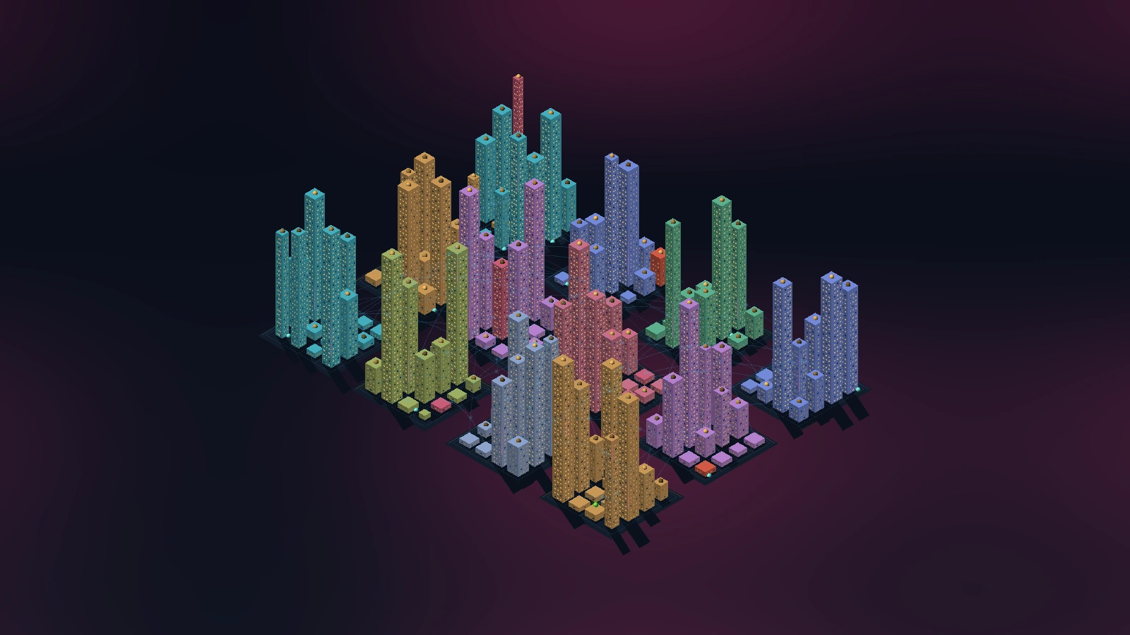
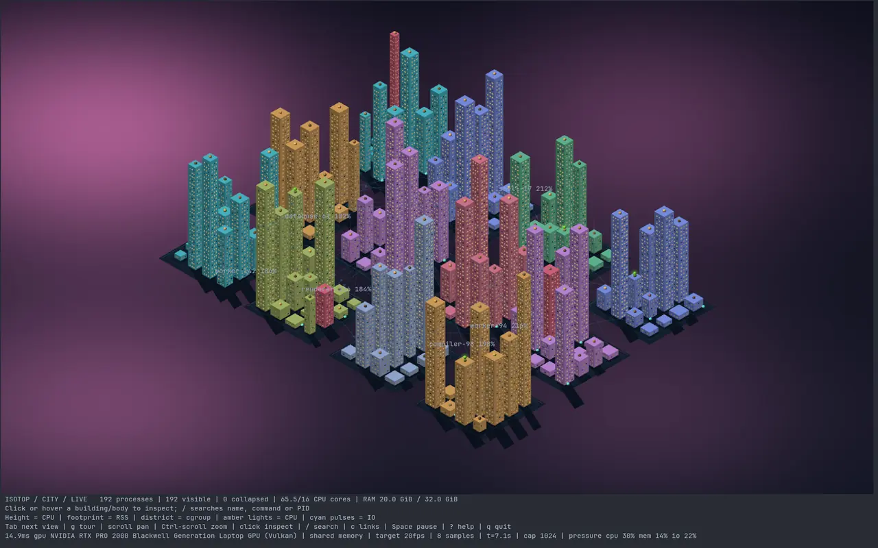
The machine as a skyline. Each process is a building on a fixed plot; its height is its CPU use, its footprint is its resident memory, and its district is the service (cgroup) it belongs to. Windows glow with activity, rooftop lights pulse on busy buildings, and the whole thing is seen through an orthographic isometric camera, so the vertical axis is drawn at the same scale as the ground. It is the first view (1, or the default of --view) and the plainest: a 3D bar chart arranged into neighbourhoods. It is also deliberately not a treemap, and the reason it is not is the most interesting thing about it.

The system being modelled

A city is a good picture of a process table because the two share a structure. Land is divided into parcels by a cadastre that does not change when a building does: a plot keeps its address while the building on it is torn down and rebuilt. Parcels are gathered into districts, which is how a services table is organised (a service owns its processes). Buildings differ in how much ground they take (a footprint) and how high they reach, and the eye reads a skyline instantly as a distribution: many low blocks, a few towers. Software visualisation has used the metaphor for a long time (Wettel and Lanza, CodeCity, 2007: packages as districts, classes as buildings, methods as height); isotop borrows it for a live system.

Why not a treemap? The standard tool for "a hierarchy with a size at each leaf" is the treemap (Johnson and Shneiderman 1991; Shneiderman 1992): fill a rectangle, divide it among the children in proportion to their sizes, recurse. It is space-filling and encodes size as area. Two properties make it a poor fit here:

• Instability. Slice-and-dice and squarified layouts (Bruls, Huizing and van Wijk 2000) place every cell as a function of every other cell's size. When the sizes are sampled once a second and change by percent each time, the layout reshuffles continuously; the cure literature (ordered treemaps, Shneiderman and Wattenberg 2001) reduces but does not remove it. isotop's invariant is the opposite: a process keeps its place when CPU, memory or the population changes (Theory Stable Layout).
• Area is a weak channel. Cleveland and McGill (1984) ranked the elementary perceptual tasks by accuracy: position along a common scale, then along non-aligned scales, then length, direction and angle, then area, then volume and shading. An area-coded value is read less accurately than a length-coded one, and the quantity that changes fastest, CPU, deserves the better channel.

The City is closest to a quantum treemap (Bederson, Shneiderman and Wattenberg 2002): every leaf occupies exactly one fixed-size cell, a quantum, and the data are carried by something other than the cell's area. Here the cell is the 4 by 4 plot, and the data go into the third dimension (height) and into the size of the building inside its plot.

History

The thing City draws is the planned city: land divided into equal parcels before anyone builds on it.

• Rectilinear street plans are older than any name attached to them. Excavated cities of the Indus valley such as Mohenjo-daro (third millennium BCE) show blocks laid out on a grid, and Greek colonies used regular plots from the seventh century BCE onward. Historians treat "the first grid" as an unanswerable question.
• The tradition names Hippodamus of Miletus (fifth century BCE) as its inventor, on the authority of Aristotle, who says in the Politics that Athens had him plan the Piraeus. Modern scholarship disputes the invention and the attribution of other cities to him, and some argue his real contribution was theoretical: a division of a city into classes of land and people. Aristotle also records that he wore his hair long, wore costly ornaments, and dressed in the same cheap warm cloak in winter and summer.
• Roman town planning combined a rectilinear grid with a forum at its centre and a wall around it, and carried the plan across the empire. The Spanish crown's colonial ordinances of the sixteenth century did the same for a new continent (the grid-and-plaza pattern of Spanish American towns).
• Two nineteenth-century plans are the usual modern exhibits. The Commissioners' Plan of 1811 laid a grid of avenues and numbered streets over Manhattan above Houston Street, on a survey by John Randel Jr., and critics have objected to its rigidity ever since. Ildefons Cerda's plan for the Eixample of Barcelona (late 1850s) also drew on the Hippodamian model, with equal blocks and chamfered corners, and was much altered by landowners and speculation afterwards.
• The step from the plan to the metaphor in software is recent: Wettel and Lanza's CodeCity (2007) drew classes as buildings and packages as districts. City differs from that line in one respect it shares with the cadastre, not the skyline: a parcel keeps its address when the building on it changes.
• Nobody has yet determined whether a district of sixteen is closer to a Roman insula or to a block of the Eixample; the tallest buildings in both are the exceptions.

Theory

Perceptual ranking and the choice of channel

Stevens (1957) modelled the apparent magnitude of a stimulus as a power law of its physical magnitude, $\psi = k,\phi^{\beta}$, with exponents commonly quoted near 1.0 for length, about 0.7 for area and 0.6 for volume (later studies put the area exponent anywhere from 0.7 to 0.9; treat the figures as order of magnitude). A building's height is a length, read against the ground at its foot; its footprint is an area. The City therefore puts the fast, important quantity (CPU) on the length channel and the slow, heavy-tailed one (memory) on the compressive area channel. That is my reading of the design; the code comments say only that "idle processes stay low blocks; one busy core is a ~23-unit tower and multi-core work climbs towards 45, against 4-unit plots".

Two caveats the ranking does not cover. First, the bars are in three dimensions, and in 3D the bases are at different screen heights, so the comparison is a length on non-aligned scales, which Cleveland and McGill rank below position on a common scale. Second, occlusion: at isometric pitch ($\arcsin(1/\sqrt3) = 35.26^\circ$, render::ISOMETRIC) a tower of height $h$ hides the ground behind it for a distance $h/\tan(35.26^\circ) = 1.414,h$ along the view direction. A one-core tower (23 units) hides 32.5 units, eight plots, of what stands behind it; a district is 16 units wide and districts are 23 apart. That is why the camera rotates (Q, e), tilts (PgUp, PgDn) and flips top-down (t).

Orthographic isometric projection

Camera::view maps a world point $(x, y, z)$ to the screen with a parallel projection. With elevation $\theta$ (pitch) and the world turned 45 degrees, the horizontal screen coordinate is $(x - y)/\sqrt2$ and the vertical one is $\big((x+y)\sin\theta/\sqrt2 - z\cos\theta\big)$, both multiplied by SCALE $= \sqrt{3/2}$. At the isometric $\theta$, $\cos\theta = \sqrt{2/3}$, so a unit of height is exactly one pixel at zoom 1, and so is a unit step along either ground axis (the three axes meet at 120 degrees and have equal length). There is no vanishing point: equal heights draw equal, wherever they stand, which is what a bar chart needs. See also Theory Camera and Projection and the figure there on the camera's axes.

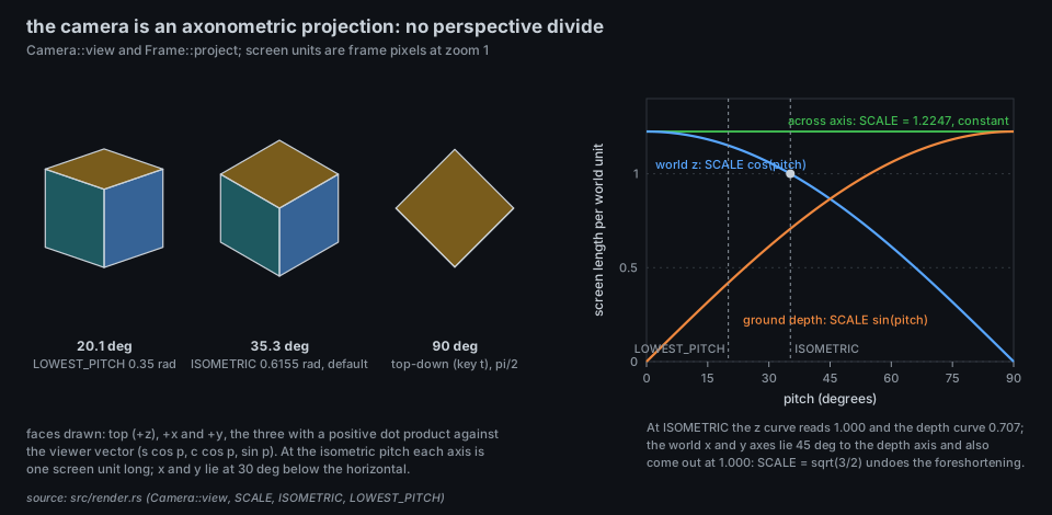
Tilting to the lowest allowed pitch (LOWEST_PITCH = 0.35 rad, 20 degrees) stretches a unit of height to $\cos(0.35)\cdot1.2247 = 1.15$ pixels; top-down ($\pi/2$) removes height from the picture altogether and leaves the plan: footprints and district colours only.

Saturating scales: the numbers behind the curves

Both data channels pass through a rectangular hyperbola $b(u, K) = u/(u+K)$ (model::bounded), the Michaelis-Menten form: linear near zero with slope $1/K$, half of its maximum at $u = K$, and bounded by 1.

• Height $= \big(1 + 44,b(\mathrm{cpu},100)\big)\cdot\mathrm{grow}$ world units, CPU in percent of one core (100 is one core), so a busy core is half-height: 23 units, 5.75 plots. The asymptote is 45 units (11 plots).
• Half-side $= \big(0.42 + 1.05\sqrt{b(\mathrm{MiB},220)}\big)\cdot(0.35 + 0.65,\mathrm{grow})$, so the building is a square of side $2\times$ that: 0.98 units at 1 MiB, 2.33 at 220 MiB, 2.75 at 1 GiB, at most 2.94 at the limit, inside a 4-unit plot (a 54% fill at most).

What resolution does the display keep? The derivative of height is $44,K/(u+K)^2$ units per percent: 0.44 at zero, 0.11 at one core, 0.0176 at four cores. At the default zoom of 5 (5 pixels per unit) one pixel of height is therefore worth 0.45% CPU near idle, 1.8% at one core and 11% at four cores; above about 400% the display no longer separates neighbours. For memory the footprint takes the square root of an already saturating function and adds a constant floor so tiny processes do not vanish:

memory	side (units)	area (units squared)	area against 1 MiB
1 MiB	0.98	0.96	1.0
12 MiB	1.32	1.74	1.8
100 MiB	2.01	4.06	4.2
1 GiB	2.75	7.54	7.8
16 GiB	2.93	8.56	8.9

A factor of 1000 in memory (1 MiB to 1 GiB) is a factor of 7.8 in area, 2.8 in side. With the Stevens exponent of 0.7 for apparent area the viewer would perceive $7.8^{0.7} = 4.2$. The footprint is a rank and order of magnitude cue, not a measurement; read the number off the inspector.

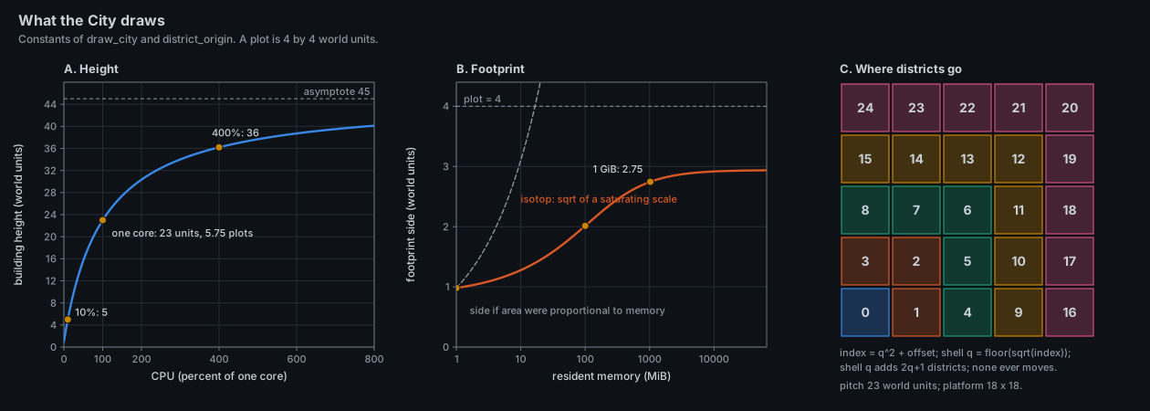
Panel C is the district fill order described under How isotop realises it.

Mapping

Visual element	Measured quantity (platform source)	Transform	Status
Building height	CPU per cent of one core (Linux: /proc/<pid>/stat utime+stime ticks; macOS: Mach time), counter delta over the sample interval	$\tau = 1.5$ s exponential smoothing in model::measure, then $\tau = 0.3$ s in Scene::ease; $1 + 44,u/(u+100)$	measured, smoothed
Footprint (square)	resident memory (Process::memory: RSS on Linux, physical footprint on macOS), eased by $\tau = 0.3$ s	$2,(0.42 + 1.05\sqrt{m/(m+220)})$, $m$ in MiB	measured, compressed
District	Process::group: Linux, the nearest .service or .scope of the unified cgroup path (else the last path component, else "ungrouped"); macOS, the outermost .app bundle or the executable name	one 16-plot block per 16 members	measured grouping
Plot within a district	none	lowest free slot of 16 at the time of arrival, row-major	decorative (arrival order)
District colour	none	DISTRICTS[district_index % 8] (8 colours, cycling): a district with more than 16 members is several blocks of different colours	decorative
Pink / orange / red building	process state Z / T or t / D	replaces the district colour	measured; no D on macOS
Wall shading	none	four sides at 0.40, 0.66, 0.55, 0.30 of the colour, roof at 0.95	decorative lighting
Cast shadow	the height	dark quad skewed by $(0.5, 0.3)\times\min(h, 14)$	decorative, redundant with height
Windows (only at zoom above 3)	CPU for brightness; height for the count	$\lfloor h/0.85\rfloor$ rows of 3 per wall; 1 in 5 unlit by an arithmetic pattern of pid, row and column; lit brightness $0.55 + 0.35,u/(u+50)$	count redundant with height, brightness measured, which ones are lit decorative
Amber rooftop light	CPU above 1%	a pulsing sphere, $0.65 + 0.25\sin(2t + \mathrm{pid})$	measured on/off; pulse decorative
Green beacon	NVIDIA per-process GPU memory present (NVML)	glow and sphere on the roof	measured; absent on macOS
Cyan pulse at the foot	storage I/O rate above 1024 bytes per second (Linux /proc/<pid>/io; macOS rusage)	a sphere sliding along the building's base edge	measured on/off
Arcs and pink beams	socket links; connections leaving the machine	arcs lifted 1.5 above the roof, as in Orbit	measured
Rise on birth	a process appearing	height and footprint grow over 0.9 s (cubic ease-out)	measured event
Ring on exit	a process vanishing	an expanding ring and glow where it stood, 1.2 s	measured event

How isotop realises it

City is a ViewModule in src/views/city.rs: the state struct City owns the seating, and City::draw calls City::place to seat every admitted process before drawing the districts and buildings. Its registry row in views::REGISTRY builds it with a closure (Box::new(city::City::default())), so Scene holds no City state.

Seating. City keeps plots (identity to district and slot), groups (group name to its districts, in order) and occupancy (per district, slot to identity). A process already seated keeps its plot. A newcomer scans its group's districts in order for the lowest free slot of 16; if none, it opens a new district at the end. A process that exits frees its slot (occupancy[district].remove), which the next newcomer of the same group will take. District blocks are never freed, so a district's index and place never change. Admitted processes are visited in Identity order (pid, then start time), so on a cold start the seats are in pid order. The slot $s$ of a district is at plot $(s \bmod 4,\ \lfloor s/4\rfloor)$, 4 units apart, building centred in it.

Where districts go. district_origin(index) fills square shells: with $q = \lfloor\sqrt{\mathrm{index}}\rfloor$ and $o = \mathrm{index} - q^2$, the grid cell is $(q, o)$ for $o \le q$ and $(2q - o,\ q)$ otherwise, times a pitch of 23 units. Shell $q$ adds $2q+1$ districts to the L-shaped border of the previous square, so index 0 is the grid cell $(0,0)$, 1 is $(1,0)$, 2 is $(1,1)$, 3 is $(0,1)$, 4 is $(2,0)$, and no district ever moves; twelve districts make a complete $4\times3$ rectangle. Each district is an 18-unit platform (a 16-unit block plus a margin of one) with a 5-unit street between neighbours.

Time. Resource figures come eased (Scene::ease: $\alpha = 1 - e^{-\Delta t/0.3}$ towards the sampled CPU and memory, reset after a gap longer than 2 s or a rewind), so a 1 s sample step is smoothed into continuous motion at the frame rate. The easing is frame-wide and every view reads the same figures through Stage::resources. City uses stage.time for its animations and does not step anything with stage.dt.

Growth. simulation::growth is a cubic ease-out over GROW_SECONDS = 0.9 s, applied as height $\times\ \max(\mathrm{grow}, 0.05)$ and half-side $\times\ (0.35 + 0.65,\mathrm{grow})$. Headless renders and tests start fully grown; the interactive app sets Scene::intro so the processes already running when it starts bloom as well.

Draw order and picking. Platforms and grid lines, then for each building a shadow, four walls (and windows), the roof, the rooftop light, the beacon and the I/O sphere. Walls, windows and roof carry the process index into frame.identities; platforms and shadows carry NONE. positions[id] is the plot centre on the ground, which is what the tour, labels and the exit flash read. The depth buffer resolves occlusion; the pick buffer follows, so a click lands on whatever building is in front.

Fit. Scene::fit frames the districts' ground positions and leaves vertical headroom of $\max(24,\ \text{tallest}\cdot\cos(\text{pitch})\cdot\sqrt{3/2} + 8)$ world units, where tallest is the tallest building of the last frame, which City::draw writes back through Stage::headroom.

CPU and GPU. Everything is quads, lines and sphere impostors on the shared display list, so there is no special parity case.

Stability. The harness checks the contract and the City has no waived property: city_does_not_relocate_when_resources_or_population_change and the shared harness enforce it, and focusing a subtree or lowering --limit hides buildings but frees no plot (clearing the focus restores them).

What degrades where. No optional source is read (the view declares none): the demand is empty. Without NVML there are no green beacons. On macOS state D is never reported, memory is the physical footprint, districts are app bundles, and there is no GPU beacon; everything else is as on Linux. When cgroup v2 is missing on Linux, Process::group is still the service named in /proc/<pid>/cgroup.

Reading the picture

What the demo render shows (--demo --view city --width 1600 --output ...): twelve districts forming a $4\times3$ rectangle (the first four shells of the L-shaped fill), each a 4 by 4 block of sixteen buildings in one colour on a dark platform. Each district is a mixture of towers and low blocks. That matches the demo workload: its CPU is $((1+\sin\varphi)/2)^4$ times $20 + 24,(i \bmod 9)$ percent (plus 110 for every 47th process), which at --time 12 has a median of about 5.7% (a block under one plot tall), a mean of about 32% and a maximum of 312% (a tower of 8.6 plots). Pink, orange and red buildings are zombie, stopped and blocked processes. Rooftops carry small amber lights; walls carry rows of warm windows; faint cyan arcs link some buildings. The surroundings are a violet dusk sky whose haze reflects the demo's pressure.

You can infer

• The ranking of CPU between processes, from height, with the best accuracy in the lower half of the curve (below one core).
• Order of magnitude of memory, and the biggest of a district, from the footprint.
• Who belongs together: the district.
• State anomalies: colour overrides make stuck (red), stopped (orange) and zombie (pink) processes stand out.
• Births and exits: a rising building and an expanding ring.

You cannot infer

• Instantaneous CPU. The height is an exponential average (1.5 s, then 0.3 s) of a tick delta over the sample interval (1 s by default); a 100 ms burst does not appear. The first sample of a new process carries no CPU rate and is drawn at the floor (the code leaves cpu at 0).
• CPU above about 400%. The curve saturates; multi-core work looks alike beyond it.
• Memory exactly. A building at 1 GiB is only 2.8 times as wide as one at 1 MiB.
• Anything from the position within a district or from the colour of a district. Both are arrival order and a cycling palette.
• Which window is lit. The pattern comes from a hash of the pid and a level and column index.
• What stands behind a tall building. Rotate or go top-down.
• Age. Pid order seeds the slots at start, but slot reuse scrambles it.

Resolution. A 1600-pixel render fits about twelve districts, so a building is on the order of 20 to 30 pixels wide and a one-pixel step in height is about 0.5% CPU near idle (zoom 5); the terminal's own cell grid is coarser, but with SGR-pixel mouse reporting (Ghostty, Kitty) hover is pixel-exact.

Try it

./target/release/isotop --demo --view city
./target/release/isotop --demo --view city --width 1600 --output city.png --renderer cpu
./target/release/isotop --demo --view city --processes 600 --width 1600 --output big.png
./target/release/isotop --view city                       # live

Keys: 1 selects it; t toggles top-down and isometric; Q and e rotate a quarter turn; PgUp and PgDn tilt; Ctrl-scroll zooms (windows appear above zoom 3); f focuses the selected process and its descendants (the rest are hidden, not moved); c cycles the link arcs; click selects, hover names. --limit N caps admitted processes (default 1024).

Where in the code

• src/views/city.rs: City, City::place, City::draw, district_origin, draw_district, draw_building, draw_windows, Plot; tests city_does_not_relocate_when_resources_or_population_change.
• src/render.rs: Scene::fit, Scene::ease, admitted, Stage::headroom.
• src/model.rs: bounded, measure (CPU rate and its smoothing), Process.
• src/palette.rs: DISTRICTS, process_color, tint.
• src/simulation.rs: growth, GROW_SECONDS, smoothing.
• src/views.rs: the city row (LinkRule::All, link_lift 1.5, Backdrop::Dusk); the legend is City::legend.
• src/platform/linux/mod.rs: cgroup_name, classify; src/platform/macos/logic.rs: group.
• Figure script: docs/figures/city-encodings.py.

Variations and open questions

• A second channel for the same height. Split each tower into a lower part for kernel time and an upper one for user time: Process::system_share already carries the split (Linux and macOS). A tower that is mostly system time is a different animal from one that is mostly user time.
• Honest area. Make the footprint area proportional to memory over a bounded range (say a logarithm over 1 MiB to 16 GiB) and let the plot grow with the district when a process exceeds it: a true quantum treemap with variable quanta. What does the stability invariant cost?
• Hue for memory. Reserve the walls' lightness for memory rank and put the district identity in the platform colour only, so footprint is a redundant channel with a better-known ordering (lightness is rank-ordered; hue is not).
• Resolve the saturation. Replace the hyperbola by $\log(1+u/K)$ above one core so multi-core work separates; compare the histogram of the displayed variable (an entropy view of the transform): the best transform for a heavy-tailed variable maps its quantiles evenly onto pixels.
• Windows that mean something. Make the lit count proportional to thread count or to runnable threads; at present they are texture.
• Open: is 16 the right quantum? A cgroup of 17 processes costs a whole 16-plot district, almost empty. Cells of 12 or 25 would trade the look of a square block against waste.

References

• B. Johnson and B. Shneiderman, "Tree-Maps: a space-filling approach to the visualization of hierarchical information structures", Proc. IEEE Visualization '91 (1991), 284-291.
• B. Shneiderman, "Tree visualization with tree-maps: 2-d space-filling approach", ACM Transactions on Graphics 11(1) (1992), 92-99.
• M. Bruls, K. Huizing, J. J. van Wijk, "Squarified treemaps", Data Visualization 2000 (Springer, 2000), 33-42.
• B. Shneiderman and M. Wattenberg, "Ordered treemap layouts", Proc. IEEE Symposium on Information Visualization (2001), 73-78.
• B. B. Bederson, B. Shneiderman, M. Wattenberg, "Ordered and quantum treemaps: making effective use of 2D space to display hierarchies", ACM Transactions on Graphics 21(4) (2002), 833-854.
• W. S. Cleveland and R. McGill, "Graphical perception: theory, experimentation, and application to the development of graphical methods", Journal of the American Statistical Association 79(387) (1984), 531-554.
• S. S. Stevens, "On the psychophysical law", Psychological Review 64(3) (1957), 153-181.
• J. Mackinlay, "Automating the design of graphical presentations of relational information", ACM Transactions on Graphics 5(2) (1986), 110-141.
• R. Wettel and M. Lanza, "Visualizing software systems as cities", Proc. IEEE International Workshop on Visualizing Software for Understanding and Analysis (VISSOFT) (2007), 92-99.
• E. R. Tufte, The Visual Display of Quantitative Information (Graphics Press, 1983).