View Flow

View: Flow

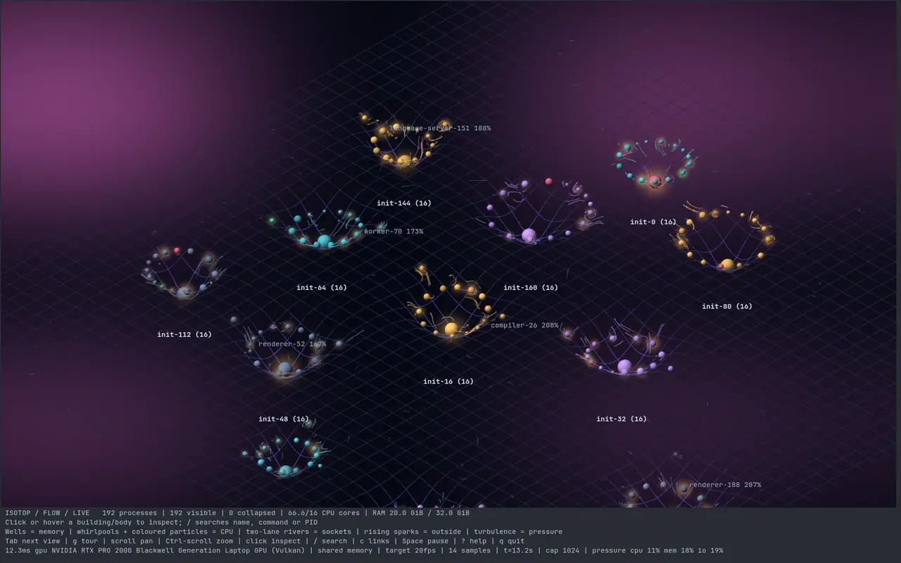
Spacetime weather. Thousands of tracer particles are carried through a velocity field painted over a rubber sheet that memory bends into wells. Each solar system of the Orbit layout bends a bowl as wide as the system and deeper for more memory; busy processes stir whirlpools and shed particles in their colour; socket links become two-lane rivers between the processes that talk, one lane each way; connections that leave the machine send sparks rising off the sheet; exits burst outward; pressure adds turbulence. It is the fourth view (4), and the one whose picture is most easily misread as physics. This page says exactly what is solved, what is drawn, and where the "gravity" is a metaphor.

The short version of the truth: Flow integrates a first-order system, $\dot{\mathbf{x}} = \mathbf{u}(\mathbf{x}, t)$, for massless tracers in a field built from analytic pieces (vortices, jets, a weak inflow and a turbulent background). There are no forces, no momentum and no energy. The wells are drawn, and the particles ride them up and down, but the slope does not push them.

The system being modelled

Two real things are being imitated at once.

A weather map of fluid flow: a velocity field and the paths of tracers in it. Visualising a flow by releasing particles and drawing their recent tracks is as old as smoke-tunnel and dye photography; the computer version integrates $\dot{\mathbf{x}} = \mathbf{u}$ and draws a short trail. Three curves are easy to confuse. A streamline is tangent to $\mathbf{u}$ at one instant; a pathline is the track of one particle through time; a streakline joins all the particles released from one point. For a steady field all three coincide; for an unsteady one they do not. Flow's trails are pathlines, and its field is steady for 0.25 s at a time (it is rebuilt that often) with a time-dependent turbulent term on top.

A gravity well on a rubber sheet: the standard teaching picture of general relativity (a mass dents a sheet; a marble rolls in). The picture is an embedding diagram of space; the textbook case is Flamm's paraboloid for the Schwarzschild spatial geometry (Flamm 1916), a surface of revolution $z = 2\sqrt{r_s(r - r_s)}$ whose wells get arbitrarily steep. isotop's wells are Gaussians, bounded and smooth, and the "marble" is not pulled down them. Treat the sheet as a depth gauge. (For an honest treatment of the real object, see Math Schwarzschild and Horizon.)

History

The thing Flow draws is a flow made visible by tracers, over a surface that is also a picture of gravity.

• Osborne Reynolds's experiment of 1883 injected dye into water running through a glass tube: at low speed the dye held a straight thread, and above a threshold it broke into eddies. The dimensionless number named after him came out of that comparison of regimes.
• Ludwig Prandtl's group at Gottingen filmed flows in water channels by scattering particles on the surface (aluminium powder, mica or lycopodium spores). The films date from around 1930 and were made largely for teaching, to show flow separation. Early on the exposures were so short that the particles appeared as dots, not the expected streaks, and the team changed to a camera with a longer exposure. Modern researchers at DLR later analysed the old films with particle image velocimetry and recovered the vortex strengths and speeds that Prandtl could not measure.
• The terms Flow uses, streamline, pathline and streakline, name three different curves that coincide only in a steady flow. Dye photographs show streaklines; a long photographic exposure of particles shows pathlines.
• The wells come from a different history. Ludwig Flamm's paper of 1916 embedded the spatial geometry of Schwarzschild's solution as a surface of revolution, now called Flamm's paraboloid. It is a rigorous picture, and sources that discuss it note that the popular rubber-sheet analogy resembles it only superficially and is a common source of misunderstanding. I did not trace who first drew the rubber sheet ((unverified)).
• Vortex blobs, the regularised vortex Flow uses, come from the numerical work of Chorin (1973), cited below. The Plummer sphere that softens the inflow was introduced for globular clusters (1911).
• Flow combines a flow-visualisation tradition and a cosmology teaching picture that were never meant to meet, and the tracers do not fall into the wells.

Theory

Elementary flows

Flow's velocity field is a sum of elementary two-dimensional flows. With $\mathbf{d} = \mathbf{x} - \mathbf{c}$ and $d = \lvert\mathbf{d}\rvert$:

• Core-regularised vortex at $\mathbf{c}$, strength $\Gamma$ (a signed velocity-times-length) and core radius $r_c$: $$ \mathbf{u}v = \frac{\Gamma}{d^2 + r_c^2},(-d_y,\ d_x), \qquad u\theta = \frac{\Gamma,d}{d^2 + r_c^2}. $$ Close in it is solid-body rotation, $u_\theta \approx (\Gamma/r_c^2),d$; far out it falls as $1/d$, the irrotational vortex of potential flow with circulation $2\pi\Gamma$. The speed peaks at $d = r_c$, at $\Gamma/(2r_c)$. The vorticity is $2\Gamma r_c^2/(d^2+r_c^2)^2$, a smooth bump. This is the algebraic core of the vortex-blob methods (Chorin 1973) that replace the point vortex's $1/d$ singularity with something integrable; Lamb (1932) and Saffman (1992) have the family (Rankine, Lamb-Oseen and the rest). The field is divergence-free: $\partial_x u_x + \partial_y u_y = 0$.
• Softened inflow. $\mathbf{u}_s = -Q,\mathbf{d}/(d^2 + w^2)^{3/2}$ is the gravitational field of a Plummer sphere (Plummer 1911), $\mathbf{g} = -GM,\mathbf{d}/(d^2+\epsilon^2)^{3/2}$, with $GM \to Q$ and $\epsilon \to w$. Used as a velocity rather than an acceleration, this is the overdamped limit of motion in a potential: $\dot{\mathbf{x}} \propto -\nabla\Phi$, a gradient flow with no orbits. Its maximum speed is at $d = w/\sqrt2$ and equals $0.385,Q/w^2$.
• A jet lane $\mathbf{u}_j = \mathbf{\hat t},S,e^{-\ell^2}\sqrt{\sin(\pi s/L)}\ \mathrm{sgn}(n)$, along a segment of length $L$ with along-coordinate $s$, signed cross-coordinate $n$ and lane coordinate $\ell = (\lvert n\rvert - 0.6,w_j)/(0.5,w_j)$. The sign flips across the centreline: two opposite streams side by side, a shear layer, where the tangential velocity jumps by $2S e^{-1.44}$ across $n = 0$. In a real fluid that vortex sheet would roll up (Kelvin-Helmholtz); in a prescribed field it just sits there, and the grid smooths it.
• Turbulence $\mathbf{u}_t = A,(\sin(0.31,y + 0.8,t),\ \cos(0.29,x - 0.6,t))$: two crossed travelling shear waves of wavelength about 20 world units and periods 7.9 s and 10.5 s. Each component depends on the other coordinate, so it is divergence-free too.

Hamiltonian structure and the integrator question

A two-dimensional, incompressible flow is a Hamiltonian system: with a stream function $\psi$ such that $u_x = \partial_y\psi$ and $u_y = -\partial_x\psi$, a tracer obeys $\dot x = \partial_y\psi$, $\dot y = -\partial_x\psi$, i.e. Hamilton's equations with $\psi$ as the Hamiltonian and $(x, y)$ as the conjugate pair. For one vortex, $\psi = \tfrac{\Gamma}{2}\ln(d^2 + r_c^2)$: the conserved quantity of a tracer is its distance from the vortex. Any good integrator should keep a tracer on its circle. The phase space is the plane itself, so "energy" is $\psi$, and a method either drifts in $\psi$ or does not.

Flow integrates each particle with the explicit midpoint (RK2) method:

$$ \mathbf{k}_1 = \mathbf{u}(\mathbf{x}_n), \quad \mathbf{k}_2 = \mathbf{u}\big(\mathbf{x}_n + \tfrac{\Delta t}{2}\mathbf{k}_1\big), \quad \mathbf{x}_{n+1} = \mathbf{x}_n + \Delta t,\mathbf{k}_2 . $$

Apply it to rotation at angular rate $\Omega$, $\dot z = i\Omega z$, and put $\zeta = \Omega,\Delta t$. One step multiplies $z$ by the stability function $R(i\zeta) = 1 + i\zeta - \zeta^2/2$, of modulus

$$ \lvert R\rvert = \sqrt{1 + \zeta^4/4} > 1 . $$

Explicit Euler has $\sqrt{1+\zeta^2}$, the classical fourth-order Runge-Kutta $\lvert 1 + i\zeta - \zeta^2/2 - i\zeta^3/6 + \zeta^4/24\rvert < 1$ for $\zeta \lesssim 2.8$, and the implicit midpoint rule $(1 + i\zeta/2)/(1 - i\zeta/2)$ has modulus exactly 1: it is symplectic, and for a linear rotation it keeps the radius to rounding. RK2 midpoint is not symplectic and not area-preserving: its map expands area by $1 + \zeta^4/4$ per step, so a tracer spirals outwards at a rate $\approx\zeta^4/8$ per step for small $\zeta$ and catastrophically once $\zeta \sim 1$. Euler's error is of order $\zeta^2$ and equally one-sided; for $\zeta \lesssim 0.3$ the midpoint rule's drift is negligible (1.0005 per step at 0.25).

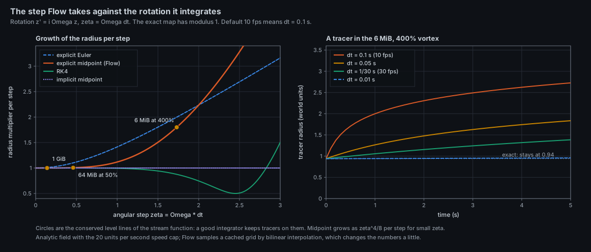
How big is $\zeta$ in practice? The step is dt = clamp(time - flow.time, 0, 0.1): at the default --fps 10 it is 0.1 s, at 30 fps 0.033 s, and slower frame rates are clamped (the flow runs in slow motion, not in big steps). The core rotation rate is $\Gamma/r_c^2$. I computed three cases from the formulas in weather (strength $6 + 60,u/(u+40)$ with the sign by pid parity, core radius $r_c = 1 + 2r_b$ with $r_b$ the body's mass_radius of its subtree):

process	$r_b$	$r_c$	$\Gamma$	$\Omega_0 = \Gamma/r_c^2$	peak speed	$\zeta$ at $\Delta t = 0.1$	growth per step
6 MiB at 400%	0.44	1.87	60.5	17.3 rad/s	16.2	1.73	1.80
64 MiB at 50%	0.96	2.92	39.3	4.6 rad/s	6.7	0.46	1.006
1 GiB at 100%	2.42	5.84	48.9	1.4 rad/s	4.2	0.14	1.0000

Measured with a stdlib port of the field and of Flow::advance (analytic field, speed capped at 20 as in weather): for the first case, tracers started anywhere from 0.3 to 1.9 units from the centre end up at radius 2.7 to 2.8 after 5 s at $\Delta t = 0.1$ (they are centrifuged out of the core within a handful of steps), at 1.0 to 2.0 at $\Delta t = 1/30$, and stay near their starting radius at $\Delta t = 0.01$ (drift under 0.1 at the innermost start; this last run used the neighbouring parameters $\Gamma = 60.5$, $r_c = 1.5$). The other two cases are unaffected. Sampling the cached field on the grid by bilinear interpolation (cells of 0.7 to 2.5 units) changes the numbers a little and leaves the effect in place. Consequence for the picture: at the default frame rate, a small process at high CPU, the busiest kind of thing in a real session, has a hollow vortex core, a ring of particles at about 2.7 units rather than a swirl down to the pebble. Heavy processes (large $r_b$, so large $r_c$, so small $\Omega_0$) do not show it. Particles live only 4 to 7 s, which hides the long-term drift of the outer, slower parts of every vortex.

The kick: an inertial lag

A splash or birth gives a particle a kick velocity added to the field and decayed by $e^{-2.5,\Delta t}$ each step, i.e. $\dot{\mathbf{k}} = -\mathbf{k}/\tau$ with $\tau = 0.4$ s. That is the Stokes-drag relaxation of a small inertial particle whose velocity differs from the fluid's (the leading term of the Maxey-Riley equation, Maxey and Riley 1983). A kick $k_0$ carries a particle an extra $k_0\tau$: 3.6 units for an exit's 9 units/s, 1.2 units for a birth's 3.

Gravity as a velocity

For a well of memory-proportional "mass" $Q = 0.6,r^3$ (the body radius cubed is proportional to memory), the inflow speed at its maximum is $0.385,Q/w^2$ with $w = 1 + 2r$:

body	$r$	$Q$	$w$	peak inflow
53 MiB (the smallest that gets a dimple)	0.9	0.44	2.8	0.02 units/s
1 GiB	2.42	8.5	5.84	0.10 units/s
6.4 GiB or more (the radius clamp)	4.5	54.7	10	0.21 units/s

That is 0.02 to 0.2 units per second against a turbulent background of 0.4 to 6.4 and vortex speeds up to 20. The inflow is almost inert: memory affects where particles go only through the whirlpools' core radii (which scale with the body radius) and not through the "gravity". The wells do not catch particles. The Gaussian bowls of the systems themselves (inflow = 0) act on nothing but the height at which particles are drawn.

Mapping

Visual element	Measured quantity (platform source)	Transform	Status
Body (sphere)	one process	radius $0.7\times$ mass_radius(subtree memory), at the sheet's depth plus $0.6\times$ radius	measured
Well under a system	memory of the system root's whole subtree (Layout::mass; RSS or footprint)	Gaussian bowl of depth $2 + 14,m/(m+2048)$ ($m$ in MiB), width $\max(\mathrm{extent}/2, 4)$	measured; saturating
Dimple under a heavy body	body radius above 0.9 (subtree memory above about 53 MiB)	depth $0.4,r$, width $1 + 2r$, weak inflow $0.6,r^3$	measured; the inflow is nearly inert (above)
Sheet colour	relative depth	$t = \mathrm{depth}/\mathrm{deepest}$ in the frame; colour $(28 + 70t,\ 42 + 40t,\ 72 + 120t)$: dark blue to violet	derived, relative to the frame's deepest well
Whirlpool	CPU above 0.5%	$\Gamma = \pm(6 + 60,u/(u+40))$, core radius $1 + 2r_b$	magnitude measured; handedness decorative (parity of the pid)
Particles from a process	CPU above 0.5%	$1 + 30,u/(u+40)$ per second, spawned within $1.5,r + 0.5$ of the body, life 4 to 7 s, in the process's kind colour	measured rate
River (two lanes)	socket link between two processes, its socket count $n$	width $2.5 + 0.8\ln(1+n)$; speed $(8 + 3\ln(1+n)),(0.6 + 1.4,b(u_a + u_b, 30))$; particles at $(0.4 + 0.3n),(0.5 + 2,b(u_a+u_b, 30))$ per second per end	measured count and CPU
Rising sparks	connections leaving the machine (snapshot.outside)	2 per connection per second, life 2.5 s, rising 2.5 units/s, pink	measured
Burst	an exit	40 particles at 9 units/s	measured event
Puff	a birth	12 particles at 3 units/s	measured event
Turbulence	pressure stall some avg10 of CPU, memory, I/O (Linux; macOS only the memory level)	amplitude $0.4 + 6,p/(p+25)$, $p$ = sum of the three	measured
Background tracers	none	400 per second, dim blue, life 5 to 8 s	decorative: they reveal the field
Warm and green glows	CPU, GPU memory	as in Orbit	measured

Here $b(v, K) = v/(v+K)$ is model::bounded.

How isotop realises it

Flow is a ViewModule in src/views/flow.rs; the state struct is called Wells, and its registry row in views::REGISTRY builds it with a closure. Wells owns a Galaxy (shared machinery with Orbit, in src/views/systems.rs) and an optional Flow sheet from src/medium.rs; Scene holds none of it. Wells::draw calls systems::hubs (hollow stars for unreadable parents, as in Orbit), then systems::layout, then Wells::pour, then Layout::report.

1. Layout. systems::layout(&mut self.galaxy, stage, &processes, snapshot, 0.0): the same layout code as Orbit with the orbital motion held at zero (planets sit at their starting mean anomalies, the galaxy does not turn). Each view owns its own Galaxy, so a system's centre in Flow is where Flow's galaxy placed it, which agrees with Orbit's only while neither has turned it; individual planets are not where Orbit draws them at the same moment, except at time zero. (The README says "a process sits in the same place in each"; strictly that holds for the system centres.)
2. Grid. footprint(&layout.bodies, 140), which calls render::cover: 140 cells on the longer side with a margin of $8 + 0.08\times$extent, kept if render::similar to the previous grid and rebuilt otherwise.
3. Step. dt = clamp(time - flow.time, 0, 0.1).
4. Field. weather (a free function in the module) runs when the cached field is older than 0.25 s (field_time). It zeroes the velocity and depth grids and adds, each only over the cells within its reach (around): the wells (Gaussian depth plus softened inflow), the vortices, the jets of the links; then caps every cell's speed at 20 and every depth at $-20$. The field is cached on the grid; a particle samples it by bilinear interpolation (Grid::sample).
5. Emission. Fractional rates are realised by a Bernoulli trick, while expected > random() { expected -= 1; spawn }, whose mean count is exactly expected. The random stream is one seeded XorShift32 (GOLDEN_RATIO_32), and the iterations that use it run in a fixed order (bodies in layout order, snapshot.outside sorted by identity) so a frame is repeatable. The total is capped at 6000 particles: once it is reached, room stops emission in the order of the loops (background tracers first, then bodies in layout order, then links, then sparks); only the exit bursts and birth puffs skip the check.
6. Advection. Flow::advance(dt, stir): for each particle, RK2 midpoint on $\mathbf{u}\mathrm{field} + \mathbf{u}\mathrm{turbulence} + \mathbf{k}$, then $\mathbf{k} \leftarrow \mathbf{k},e^{-2.5\Delta t}$; the trail rotates by one and its head takes the new point at the sheet's depth plus 0.15 (a rising spark gains 2.5 units/s instead). Particles are removed when their age passes their life or they leave the grid. The turbulence amplitude is $0.4 + 6,\mathrm{stir}$ with stir $= b(\text{cpu} + \text{memory} + \text{io pressure}, 25)$.
7. Draw. The sheet is a wireframe of every third grid row and column, coloured by depth; then the bodies; then, for each particle, TRAIL - 1 = 19 line segments (Frame::beam) fading along the trail with weight $s(1 - k/20)$, $s = (0.9\ \text{or}\ 0.6)\cdot\min(\mathrm{age}/0.3, 1)\sqrt{1 - \mathrm{age}/\mathrm{life}}$, and a small glow on the bright ones.
8. Time. The view takes stage.time and clamps the step itself (step 3), not stage.dt. Because the trail holds 20 positions, one per frame, a trail is $20,\Delta t$ of history: two seconds at 10 fps, two thirds of a second at 30. Streak length is local speed times that: Flow's picture is a fixed-exposure photograph whose exposure shortens as the frame rate rises.

Picking. Bodies carry their index in the pick buffer; the sheet and the particles do not. Hover names a process only over a body.

Stability. Like Orbit, Flow's layout re-places a system only when its structure outgrows the reservation (HEADROOM in systems.rs). The row waives no property; the harness checks each process's home, the centre of its system, which Wells returns from ViewModule::anchors (test-only). The flow media survive layout changes while the grid is similar.

Headless. The row's SETTLE warm-up (80 frames of 0.05 s ending at --time) lets particles fill the sheet.

What degrades. No optional source. On macOS the turbulence term sees only the memory-pressure level (0, 25 or 75); there are no green GPU glows; unreadable parents become hollow stars. Without socket links there are no rivers (and no sparks if no connection leaves the machine).

Reading the picture

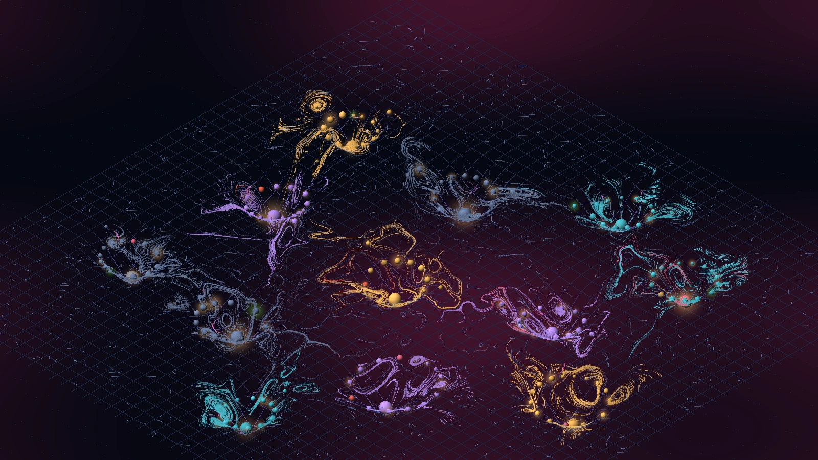
What the demo render shows: a dark violet-blue sky above a faint blue wireframe sheet, twelve bowls (one per system), each with its star near the bottom and its planets on the slopes; coloured streaks (in the kinds' colours: teal, amber, violet, slate) piled into coils around the systems, thin pink streaks where connections leave, and a field of short, dim blue streaks wandering over the flat sheet between systems. Near each star the tracks curl into closed loops; some coils look hollow, with a ring of streaks and an empty middle, which is the integrator effect described above on the small busy processes.

You can infer

• Where memory is concentrated: the deepest and widest bowls are the systems with the most memory in their trees, with diminishing returns at the top (the depth saturates, and the colour is normalised to the frame's deepest well).
• Which processes are busy: they are the ones with whirlpools and the densest particle clouds; the particle count is roughly proportional to $1 + 30,u/(u+40)$.
• Which processes talk: a river between two bodies, with its width and brightness following the socket count.
• Pressure, from the background tracers' wandering: the amplitude of turbulence rises from 0.4 to as much as 6.4 units/s.
• Births and exits, as a small burst of light-coloured streaks or a ring of 40 at 9 units/s.

You cannot infer

• Whether particles are falling into a well. They are not; the dip is a drawing.
• Handedness. A clockwise whirlpool is not different from an anticlockwise one; it is the parity of a pid.
• Absolute velocities from streak length. Streak length is speed times the trail's duration (20 frames), and so depends on the frame rate.
• Which of two overlapping systems a particle belongs to: colour is the emitter's, and the field mixes.
• The count of busy processes when many are busy. The 6000-particle cap binds in a busy session (in the demo at --time 12, 126 sources average 13.5 particles per second each; with 4 to 7 s lives and 400 background tracers per second the steady-state demand from the formulas is about 12 000 particles), and emission is then first-come in layout order, so busy processes late in the order may be starved. I did not measure the starvation; it follows from the code.
• A sheet that matches the processes' memory beyond the system level. Only the systems and the heavy bodies (above 53 MiB) have wells.
• Anything below 0.5% CPU.

Resolution. The field lives on a 140-cell grid, so features smaller than a cell or two are smoothed; the smallest vortex core (1.5 units) is about the size of a cell on a 200-unit layout. The jet lanes' centreline discontinuity is smoothed by the same grid.

Try it

./target/release/isotop --demo --view flow
./target/release/isotop --demo --view flow --width 1600 --output flow.png --renderer cpu
./target/release/isotop --demo --view flow --width 1600 --renderer gpu --benchmark 120
./target/release/isotop --demo --view flow --fps 30            # a third of the trail length in time
./target/release/isotop --view flow

Keys: 4 selects it; click a body for the inspector; f focuses a subtree; c cycles link arcs (the rivers are the flow's own depiction, so the scene's arcs show only for highlighted processes).

Where in the code

• src/views/flow.rs: Wells, Wells::draw, Wells::pour, Pour (background, around_bodies, along_links, sparks), disturb, weather, fabric, bodies, particles, footprint, Lane, PARTICLES; tests in the same file and focusing_one_process_after_another_leaves_no_orbit_or_flow_system_behind in systems.rs.
• src/views/systems.rs: layout and hubs (shared with Orbit).
• src/render.rs: cover, similar, glows, mass_radius, Stage::newborn, Stage::splashes.
• src/medium.rs: Flow (new, spawn, advance, velocity_at, depth_at), Particle, TRAIL, Grid::sample; test particles_circle_a_vortex_and_ride_a_jet.
• src/simulation.rs: XorShift32, GOLDEN_RATIO_32.
• src/views.rs: the flow row (SETTLE); the legend is Wells::legend.
• Figure script: docs/figures/flow-vortex-integrators.py.

Variations and open questions

• A symplectic or exact vortex step. Replace the RK2 step by the implicit midpoint rule or by an exact rotation about the nearest vortex: the hollow cores would fill, and the cost is a few iterations.
• Real inertial particles. Give each tracer a velocity and relax it to the field with $\tau$ (Stokes drag), plus the gradient of the sheet as a force: now the wells do pull, and tracers can be flung out of vortices by their inertia. The right integrator is then a Verlet or Boris-style kick-drift-kick.
• Let the vortices move each other. Point vortices in a plane advect one another by the Biot-Savart law and are a Hamiltonian system of their own; for four or more the motion is chaotic (Aref 1983). Letting the CPU whirlpools drift under each other's fields would make the stir dynamic.
• A real fluid. Replace the prescribed field by a stable-fluids solver (Stam 1999) forced by CPU and sockets; the shear layers between the lanes would then roll up on their own.
• Streaklines. Release particles at a point continuously and join them: a dye photograph of one process's trace.
• Fix the cap's bias. Share the 6000 budget in proportion to demand, or let each emitter's life shorten with load; check the demo for starved systems.
• Open: is there a depth profile for the wells whose slope, used as a force, gives bounded orbits of the right character (Flamm's paraboloid has none)?

References

• H. Lamb, Hydrodynamics, 6th ed. (Cambridge University Press, 1932).
• P. G. Saffman, Vortex Dynamics (Cambridge University Press, 1992).
• A. J. Chorin, "Numerical study of slightly viscous flow", Journal of Fluid Mechanics 57 (1973), 785-796.
• H. C. Plummer, "On the problem of distribution in globular star clusters", Monthly Notices of the Royal Astronomical Society 71 (1911), 460-470.
• L. Flamm, "Beitrage zur Einsteinschen Gravitationstheorie", Physikalische Zeitschrift 17 (1916), 448-454 (unverified page range).
• M. R. Maxey and J. J. Riley, "Equation of motion for a small rigid sphere in a nonuniform flow", Physics of Fluids 26 (1983), 883-889.
• H. Aref, "Integrable, chaotic, and turbulent vortex motion in two-dimensional flows", Annual Review of Fluid Mechanics 15 (1983), 345-389.
• J. Stam, "Stable fluids", Proc. SIGGRAPH '99 (1999), 121-128.
• E. Hairer, C. Lubich, G. Wanner, Geometric Numerical Integration, 2nd ed. (Springer, 2006).