Theory Model and Rates

Theory: The model, rates and smoothing

The platform samplers hand the model a list of RawProcess values: cumulative counters and instantaneous gauges. model.rs turns them into a Snapshot, the only thing the rest of the program sees. The turning is mostly one operation, differencing a counter over the time since the last reading, and one filter, an exponential smoother with a 1.5 second time constant. This page derives that filter exactly (step response, frequency response, delay), says what quantisation and aliasing do to a rate estimated this way, states the rule that makes absence a first-class value ("unknown is not zero"), and describes the budgeted selection top_n and the deterministic demo workload that every screenshot in this wiki is rendered from. The sources of the raw numbers are on Sampling on Linux and on macOS.

History

Counters and averages. Differencing a cumulative counter is how Unix has always reported CPU use: the kernel keeps totals and the tool subtracts. The smoothing is older than computers. Exponential smoothing came out of Robert G. Brown's work as an operations analyst for the US Navy in the Second World War, which he presented in 1956 for inventory demand, and of Charles C. Holt's independent report for the Office of Naval Research (ONR Report 52, 1957), which went unpublished until 2004. The idea of an exponentially decaying window is older still: Wikipedia's article on it attributes the window function to Poisson, as an extension of a numerical analysis technique from the seventeenth century. Sources differ on how much of this belongs to each man, and isotop's filter needs only the result, a weight of 1 - exp(-dt/tau) that makes the filter independent of the sampling interval.

Aliasing. The sampling theorem the aliasing section leans on is cited in the references as Shannon (1949); the folding of frequencies above the Nyquist limit is the same arithmetic whether the signal is a radio wave or a compile job.

In this project. The 1.5 s smoother is already in the first commit (2026-10-07), written inline as 1 - exp(-dt / 1.5). Making absence a value of its own, the "unknown is not zero" rule, landed on 2026-10-11 in the architecture batch #113, and the deterministic demo workload took its present form with the demo options in #120 the same day. This page derives what the constant does rather than why 1.5 was chosen, and the log does not say.

The data

Identity { pid, start } is the key for everything that persists between samples. start is a Linux starttime in ticks since boot, or a macOS start time in microseconds since the epoch; either way a recycled pid has a different start, so state keyed by Identity can never be inherited by a newcomer. Identity orders by pid then start; that total order is the tie-break in top_n, the sort order of Snapshot::processes, and the merge key of History.

Process is one row. Its fields fall into three groups:

group	fields	filled by
read directly (gauges)	id, parent, name, command, group, kind, state, memory, threads, core, cgroup, priority, nice, policy, written, started	the platform, in RawProcess::process
derived from counters	cpu, cpu_time, io_rate, read_rate, write_rate, system_share, performance_share, waiting, syscall_io, major_faults	measure in model.rs
from the background thread	files, locks_held, blocked_on, gpu_memory, and, while their sources are demanded, oom, memory_detail and thread_list (and the snapshot's links, remotes, units, pipes, unix_queues and kernel counters)	merge, by Identity (background sampler)

A field added to Process must be decided in four exhaustive struct literals (parse_stat on Linux, Sampler::process on macOS, demo_with and Transient::process in the demo): no ..Default::default(), so the compiler forces the question "what is this field where it cannot be measured?".

Snapshot is one sample: the processes sorted by Identity, memory totals, cores, elapsed (seconds on the monotonic clock since the collector started, the clock every window and history is expressed in), wall (the calendar time, seconds since the Unix epoch; in the demo DEMO_EPOCH + time), the three pressure percentages, the socket-derived links and remotes, the Cpu list, the cgroup Units, missing and sources (the two sets), the sampler's health, the life events since the previous sample, journal (the log lines delivered while it was the newest sample), the kernel counters (interrupts, softirqs, oom_kills; Pending, Pending and None until a view demands them), and observer, isotop's own row.

Measured<T> is for values measured on the background thread: Pending (not yet; before the first pass, or a process born since, or one a budget-limited scan has not reached), Unreadable (could not be read, normally for lack of permission), Known(T). A view that must tell the two apart uses it; everything else is an Option.

Collector::sample

One call, on the frame loop, in this order:

1. dt = max(now − last, 0.001) seconds from the monotonic Instants of this and the previous call.
2. System readings: pressure, memory, core count; elapsed, wall.
3. For each RawProcess of the sampler: measure(raw, previous.get(id), hz, dt), which returns the finished Process and the Counters to keep for next time. The map of kept counters is keyed by Identity and rebuilt every sample, so it only ever holds the processes alive now.
4. Per-CPU readings (Sampler::cpus(dt)), after the processes, because macOS derives its cluster clocks from the process counters just read.
5. missing, per_cluster, unreadable and shadows from the sampler; processes sorted by Identity.
6. Publish the cgroup paths and the pid → Identity map for the background thread; on the first call, start it.
7. Merge the latest background Extras.
8. Find isotop's own process (the observer).
9. If life events are demanded, drain the event queue and merge it with sample diffing (Life events); otherwise reset that state, which ends the event thread.

dt is measured at the start of the call, but the counters of the first process in the sweep are read at slightly different instants than those of the last. The error, relative to dt, is the sweep duration over --sample-ms. It is small at the default and grows as --sample-ms shrinks. It also means that the effective sampling interval is not exactly --sample-ms: the main loop checks the sample clock once per frame, so the next sample comes at the first frame boundary at or after --sample-ms, plus the duration of the sample itself. This is why rates are divided by the measured dt, never the nominal one.

Rates from counter deltas

For a cumulative counter $C$ read at $t_{k-1}$ and $t_k$, the average rate over the interval is $(C_k - C_{k-1})/\Delta t_k$. Every rate in the model is this, followed by a rule for when it is not known:

quantity	formula	None (or special) when
cpu (% of one core, may exceed 100)	$100,\Delta\text{ticks}/(\text{hz},\Delta t)$, then smoothed (below)	not an Option: reads 0.0 on a process's first sample; a backwards counter saturates to a zero raw reading
cpu_time (s)	ticks / hz	always known
io_rate, read_rate, write_rate (B/s)	$\Delta$bytes$/\Delta t$	first sample; I/O unreadable; either counter went backwards (the total would be wrong)
syscall_io (B/s and calls/s)	$\Delta/\Delta t$ for four counters	first sample; unreadable; reset; any counter backwards; always on macOS
major_faults (/s)	$\Delta/\Delta t$	first sample; reset; backwards
system_share (0–1)	$\Delta\text{system}/\Delta\text{ticks}$, at most 1	first sample; no CPU time elapsed; reset
performance_share (0–1, macOS)	$\Delta\text{perf}/\Delta\text{ticks}$, at most 1	first sample; no CPU time elapsed; a counter backwards; Linux
waiting (threads, macOS)	growth of runnable minus CPU beyond its high-water mark, per second, at most the thread count	first sample; reset; Linux
remote up, down (B/s)	per socket inode, $\Delta/\Delta t$ with $\Delta t \geq 0.1$ s since that socket was last seen	new socket; backwards; macOS (counters are placeholders)
loopback link_traffic (B/s)	per pid pair, received bytes of both ends	the first scan; absent pairs, not zeros
cgroup Unit::cpu (%)	$100,\Delta\text{usage_usec}/10^{6}/\Delta t$	first reading; counter backwards
Cpu::busy (0–1)	busy ticks over total ticks	first reading; no ticks; counter backwards
Cpu::wait	$\Delta\text{wait}_{\mathrm{ns}}/10^{9}/\Delta t$	first reading; Linux without schedstat; macOS

Counter resets

previous is keyed by Identity, so a recycled pid never meets its predecessor's counters. What can still go backwards is an exec on macOS (the new task keeps only the exec'ing thread's counters), or a counter that wraps. restarted(ticks, runnable, system_ticks, previous) is true if the CPU, kernel-mode or runnable total decreased; when it is, the rates that depend on those counters (system_share, syscall_io, major_faults, waiting) are None for that one interval, and the high-water mark of waiting starts over. The I/O counters have their own guard: IoBytes::rates uses checked_sub on the total and on each direction, returning None rather than a negative or wrapped value. The test counter_resets_read_as_unknown_rates_not_negative pins this down.

The waiting estimate deserves its caveat. macOS updates a task's runnable time only when a thread is switched on or blocks, so $\text{runnable} - \text{cpu}$ dips while threads run and recovers later. Counting only growth beyond the highest value ever seen avoids reading the dip and its recovery as waiting, and capping at the thread count bounds a first reading that was dipped by a long run.

The CPU filter

The one place the model smooths is the CPU percentage, in measure:

let raw = ticks.saturating_sub(previous.ticks) as f32 / hz / dt * 100.0;
let alpha = smoothing(dt, 1.5);              // 1 - exp(-dt / 1.5)
process.cpu = previous.cpu + alpha * (raw - previous.cpu);

with smoothing(dt, tau) = 1 − exp(−dt/τ) in simulation.rs. Write $x_k$ for raw, $y_k$ for the displayed value, $\tau = 1.5$ s.

Exactly a first-order lag

A first-order low-pass (an RC circuit) obeys $\dot y = (x - y)/\tau$. If $x$ is constant, $x_k$, over an interval of length $\Delta t_k$, the exact solution is

$$ y(t_k) ;=; x_k + \big(y(t_{k-1}) - x_k\big),e^{-\Delta t_k/\tau} \quad\Longleftrightarrow\quad y_k ;=; y_{k-1} + \alpha_k,(x_k - y_{k-1}),\qquad \alpha_k = 1 - e^{-\Delta t_k/\tau}. $$

So the code is not an approximation to the RC filter that happens to be cheap: for a held input it is the RC filter, for any interval, regular or not. That is the reason the weight depends on dt. If the sampler is paused for a minute, $\alpha \to 1$ and the display shows the average over the gap instead of lurching; if --sample-ms is changed the time constant does not.

Step response

Let the load step from 0 to 100 % at a sample instant. Then $y_k = 100,(1 - a^k)$ with $a = e^{-\Delta t/\tau}$, which is the continuous $100,(1 - e^{-t/\tau})$ read at $t = k\Delta t$. The time to reach a fraction $p$ of the final value is $-\tau\ln(1-p)$:

fraction	time after the step
63.2 %	1.50 s ($\tau$)
90 %	3.45 s
95 %	4.49 s ($3\tau$)
99 %	6.91 s

If the step falls inside an interval the first reading is partial and the output is slightly late: with the step a fraction $\varphi$ of the way into the first interval, $y_k = 100,[1 - a^{k-1}(\varphi + (1-\varphi)a)]$ against the continuous $100,[1 - a^{k-1+(1-\varphi)}]$; by the weighted AM–GM inequality the discrete value is never above the continuous one, with equality at $\varphi = 0$ and $\varphi = 1$.

Delay and frequency response

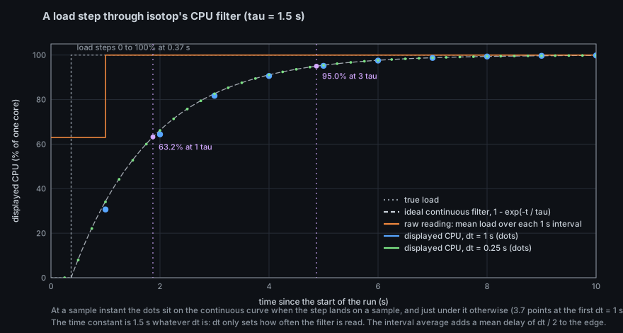
Two filters are in series: the interval average that differencing a counter implements (the mean load over the last $\Delta t$, a boxcar), and the exponential filter. The mean delay of the pair, from the true load to the displayed value, is the first moment of the combined impulse response:

$$ \bar\tau ;=; \Delta t\Big(\tfrac12 + \tfrac{a}{1-a}\Big) ;=; \tau + \frac{\Delta t^{2}}{12,\tau} + O(\Delta t^{4}), $$

using $a/(1-a) = 1/(e^{u}-1) = 1/u - 1/2 + u/12 - \dots$ with $u = \Delta t/\tau$. The $\Delta t/2$ of the boxcar and the $-\Delta t/2$ hidden in the discrete exponential cancel, so the displayed CPU lags the true load by about 1.5 s whatever the sampling interval (1.555 s at --sample-ms 1000).

In the frequency domain, from a continuous load at frequency $f$ to the displayed sequence:

$$ \lvert H_{\mathrm{box}}(f)\rvert = \left\lvert \frac{\sin \pi f\Delta t}{\pi f\Delta t} \right\rvert, \qquad \lvert H_{\mathrm{exp}}(f)\rvert = \frac{1-a}{\sqrt{1 - 2a\cos(2\pi f\Delta t) + a^{2}}}, \qquad \lvert H \rvert = \lvert H_{\mathrm{box}}\rvert,\lvert H_{\mathrm{exp}}\rvert . $$

The exponential's $-3$ dB point satisfies $\cos\omega_c = (-1+4a-a^2)/(2a)$ with $\omega_c = 2\pi f_c\Delta t$. At $\Delta t = 1$ s that is $f_c = 0.110$ Hz, against the RC value $1/(2\pi\tau) = 0.106$ Hz; at $\Delta t = 0.1$ s the two agree to four digits. The display passes slow load changes and attenuates by more than 3 dB anything faster than about one cycle every nine seconds.

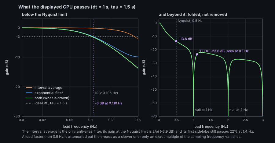
The smoother lives in the model, so every view that draws process.cpu is already filtered; the scene adds its own visual easing on top, and History records the filtered values (History).

Quantisation and aliasing

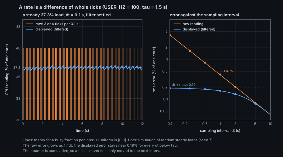
Two measurement effects sit under every CPU percentage, and neither is a bug. They are consequences of reading a counter.

Quantisation

On Linux the counter is in 10 ms ticks. Each reading $C_k$ is the true cumulative CPU time truncated to a whole number of ticks (the kernel exports $\lfloor T/q\rfloor$, $q = 10$ ms), so it carries a residue $f_k \in [0,q)$. The difference of two readings is off by $f_{k-1} - f_k$. For a load whose busy fraction per interval is spread uniformly, the residues are independent and uniform, the error has variance $2,q^2/12 = q^2/6$, and

$$ \sigma_{\mathrm{raw}} ;=; \frac{100,q}{\Delta t,\sqrt6}\ %\ \text{of one core} $$

(0.41 % at $\Delta t = 1$ s, 4.1 % at 0.1 s). For a specific steady load with $p$ the fractional part of $\text{rate}\cdot\Delta t/q$ it is $100,(q/\Delta t)\sqrt{p(1-p)}$ (a 37.3 % load at 0.1 s reads 30 or 40 %, never 37.3). Since $\overline{p(1-p)} = 1/6$, the first expression is the rms over all loads.

Because the counter is cumulative, the errors are $e_k = f_{k-1} - f_k$: they telescope. Summed over any number of intervals the error is still at most one tick, so no CPU time is ever lost, only moved to a neighbouring interval. Pushing $e_k$ through the exponential filter gives output noise

$$ \sigma_{\mathrm{exp}} ;=; \sigma_{\mathrm{raw}},\frac{1-a}{\sqrt{1+a}} ;\xrightarrow{\ \Delta t\ll\tau\ }; \frac{100,q}{\tau\sqrt{12}} ;=; 0.19\ %, $$

independent of the sampling interval. Sampling ten times faster makes each reading ten times noisier and the display no noisier at all; it only sees detail ten times finer. (Derived above and checked by simulation in the figure; the 1/6 assumes independent residues.)

Aliasing

A counter delta is an integrate-and-dump filter, and a poor anti-aliasing filter. Its gain, $\lvert\operatorname{sinc}(f\Delta t)\rvert$, is $2/\pi$ (−3.9 dB) at the Nyquist limit $f = 1/(2\Delta t)$ and has sidelobes: a load oscillating at 1.4 Hz still gets through the interval average at 22 % amplitude. Anything above the Nyquist frequency is attenuated, then folded: a load at frequency $f$ appears at $\lvert f - \Delta t^{-1}\operatorname{round}(f\Delta t)\rvert$. Only exact multiples of the sampling frequency vanish. A process that is busy for 0.4 s of every 1.02 s therefore shows a slow wobble whose fundamental has a period of about 51 s, and a 1.1 Hz oscillation of ±40 points around 50 % appears as a 0.1 Hz wobble of about ±2.6 points (after the smoother), with a ten-second period. Nothing in the displayed number can tell that from a real slow fluctuation.

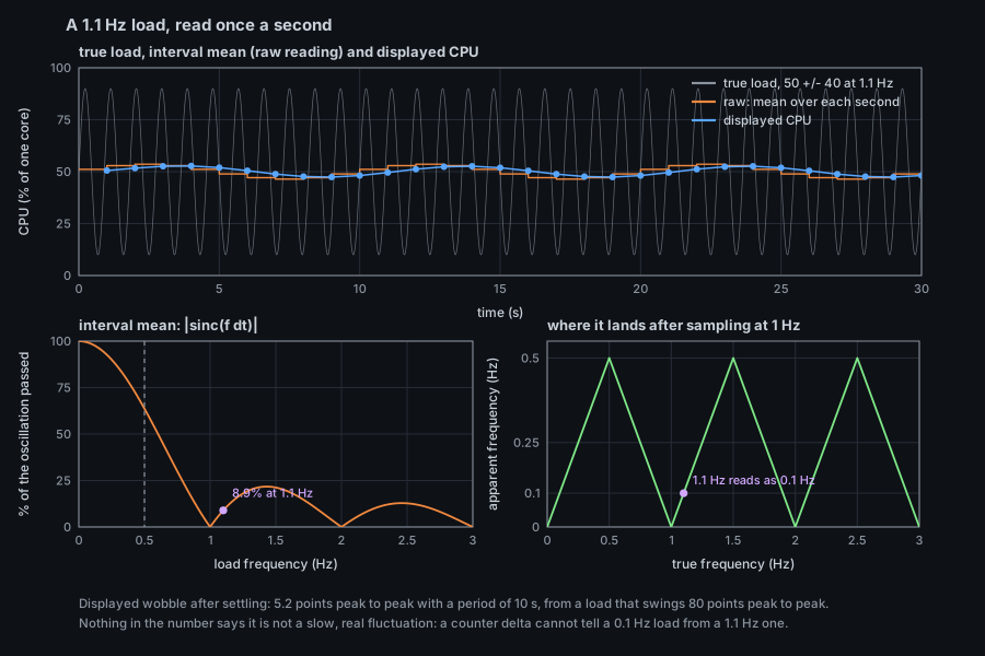
The same arithmetic applies to lifetimes: a process that lives less than the sampling interval is seen only with probability $L/\Delta t$, which is why the model has a separate event path for births and deaths (Life events).

Unknown is not zero

A reading that was not taken (the first sample of a rate, a counter that went backwards, an unreadable file) is None in the model, not 0. A zero is a measurement ("this process read no bytes"); a missing number is the absence of one, and the two draw different pictures. The contract:

• Platform samplers return None or Measured::Unreadable for what they cannot read.
• The model keeps None through every derivation (the table above).
• A view that has to draw something converts at its own boundary, unwrap_or(0.0), only to draw what it always drew. The project counts those sites as debt (unwrap_or(0 in the code report).
• What a platform never has is a Source in Snapshot::missing, so views can say "no X" instead of drawing zeros.

Honest exceptions, all in the code as it stands: Process::cpu is an f32, 0.0 on a process's first sample (the filter starts from zero, so the first few readings ramp up); the pressure percentages are 0 when a pressure file is unreadable, with missing the only record; and on macOS the remote connections carry rtt, sent and received of 0 as placeholders under Source::SocketTraffic.

top_n: a budgeted selection

top_n(processes, n, key) -> Vec<&Process> returns the n processes with the largest key, largest first. The order is total and sample-independent: ties go to the smaller Identity, and a NaN key sorts after every number (NaNs among themselves by Identity). Implementation: map to (key, process), select_nth_unstable_by to partition so the best n are in front (expected $O(N)$), truncate, then sort just those $n$ ($O(n\log n)$). Because the order never depends on input order, the same keys give the same selection in every sample, which is what lets a budgeted view change its drawn set by the data, not by hash-map iteration or the platform's listing order. Two callers use it today: Collector::sample picks the ROLLUP_PROCESSES (64) processes with the largest resident set for the smaps_rollup reads, and threads::targets orders every process by CPU, busiest first, for the thread scan. The scene's --limit admission is a separate mechanism.

describe

describe(process) -> String is the one-line "what is this" used by labels, hover and the tour. Kernel threads are matched by name prefix against a table of fourteen (kworker, ksoftirqd, migration, rcu, kswapd, irq/, …); everything else against a table of 44 known programs (systemd-journal, sshd, pipewire, ghostty, …), falling back to "app in your session", "container process" or "system service" by Kind. Matching is by prefix because comm is truncated to 15 bytes, and the table lists the more specific entries first (pipewire-pulse before pipewire, containerd-shim before containerd). It is lookup, not inference: a process named sshd that is not the SSH server gets the same label.

The demo workload

--demo replaces the whole sampler with model::demo_with(time, count, options), a pure function of time: no clock, no global state, so any time, in any order, including negative, gives the same snapshot. DemoOptions::default() gives the workload every view has always had; a view asks for more on its registry row.

• Base population. Process $i$ has pid 1000 + i, Identity::start = i + 1, a family of 16, and a kind from family % 4. CPU is scale/16 · (1 + sin θ)^4 + bonus with θ = 0.55 t + 1.71 i, scale = 20 + 24 (i mod 9) and bonus = 110 for every 47th process. Memory, I/O, priorities, open files, deleted-but-open files and file locks are fixed functions of $i$ and time. The demo does not pass through measure, so cpu here is the raw formula, unsmoothed.
• Exact CPU time (exact_cpu_time): the mean of $(1+\sin\theta)^4/16$ is $35/128$, and the integral has a closed form. With $s = \sin\theta$, $(1+s)^4 = 1 + 4s + 6s^2 + 4s^3 + s^4$, and $$\int (1+\sin\theta)^4,d\theta = \tfrac{35}{8}\theta - 8\cos\theta + \tfrac43\cos^3\theta - \tfrac74\sin 2\theta + \tfrac1{32}\sin 4\theta,$$ so CPU seconds $= \tfrac{\text{scale}}{16\cdot 0.55},[F(\theta(t)) - F(\theta(0))]/100 + \text{bonus}\cdot t/100 + 3.7,i$, exactly the integral of the displayed cpu, never decreasing. Threads are then at least $\lceil\text{peak}/100\rceil$ so a single thread never exceeds one core.
• Churn (churn): transient families (one per 16 base processes) on cycles of 24, 26, 28 or 30 s, staggered by 5.9 · family s. A parent forks one to six children over two to four seconds, each child lives 3 to 12 s and exits (one in 16 with SIGTERM, one in 16 with SIGSEGV); some leave a zombie for DEMO_ZOMBIE_SECONDS = 1 s; once per 90 s one process leaks past 1 GiB and dies by SIGKILL. Pids come from a fixed pool and are reused with a new Identity::start. demo_life lists the forks and exits in (from, to], demo_events turns them into life events (forks "from the proc connector", exits "from taskstats" with an exit record), and a test pins that the events are exactly the difference of the two populations, so splitting an interval anywhere gives the same events.
• Options for the newer sources. oom_and_memory_detail gives every process an Oom (three System processes exempt) and the 64 largest a consistent Rollup, one of them unreadable; kernel_counters synthesizes interrupts, softirqs and oom_kills (the sum of the demo units' oom_kills); threads gives every process the threads threads::demo_list synthesizes; channels synthesizes unix_queues and pipes. Plain demo leaves them all unread.
• observer synthesises isotop's own row; mortality stretches cycles to 84–105 s, adds short sh helpers, a twelve-child compile burst, a stopped unit, a victim scope that counts its OOM kills and one exit in ten that only sample diffing sees.
• Clock. DEMO_EPOCH = 1_791_605_520, 2026-10-10T04:12:00Z, is the wall time of demo time 0 (Snapshot::wall), so calendar-dependent views (the moon in the Necropolis) render the same everywhere.
• Determinism. The few random draws use Rng, seeded from hash_identity(Identity, salt) or a (family, epoch) pair, never from a global stream; salts separate unrelated uses of one identity. See Determinism. In main.rs, demo_snapshot wraps demo_with with the shown view's options and, with churn, the events between previous and time, so a live sample, a warm-up replay and a first sample all go through the same door.

What a viewer can infer

• A CPU figure is the load of the last second or so, filtered, about 1.5 s late, quantised to a tick and aliased against anything periodic near the sampling frequency.
• A memory figure is a gauge read at the sample instant.
• "No number" and "zero" are different pictures: a missing rate is skipped or marked, an idle process is a measured zero.
• A demo frame is a function of --time, not of the machine; a live frame is both.

Where in the code

• model.rs: Identity, Process, Snapshot, Measured, Collector::sample, measure, restarted, IoBytes::rates, top_n, describe, demo_with, DemoOptions, demo_life, demo_events, DEMO_EPOCH, demo_cpu_integral.
• simulation.rs: smoothing, Rng, hash_identity.
• main.rs: demo_snapshot; src/interactive.rs: the sample clock in Live::sample.
• platform/mod.rs: RawProcess.
• Figures: docs/figures/model-smoothing-step.py, model-smoothing-response.py, model-quantised-counters.py, model-sampling-alias.py.

References

• A. V. Oppenheim and R. W. Schafer, Discrete-Time Signal Processing (Prentice Hall; several editions): sampling, aliasing, the exponential (one-pole) filter and its frequency response.
• C. E. Shannon, "Communication in the presence of noise", Proceedings of the IRE 37 (1949): the sampling theorem.
• proc(5) and time(7) for the units of the counters (Linux sampling).